Dispelling Myths and Misconceptions about Modern Alternatives to Traditional PLCs: Part 3 – Programming Languages

In the first two parts we covered some basic myths and how operating system choice and setup are much more important than the choice of programming language (PL for short in this article). We’ll start this one off by addressing one of the myths from Part 1: “Myth #2: Only PLC programming languages are suitable for industrial automation.”

Let’s break that down further. What are people really trying to say when they say that? Usually, it’s any number of the following:

1. The PL needs to be simple and easy
2. It needs to be visual (e.g., ladder) to facilitate ease of use and debugging
3. It needs to be reliable
4. It needs to be fast
5. It needs to be deterministic / run in real-time, especially for safety applications

Let’s address each of these:

#1 – Simple and easy:

For a PL to be simple and easy, it should be easy to read (not cryptic; reads like natural language) and learn (shallow learning curve). A lot of these discussions have been focusing on the Python programming language, and for good reasons: Python is not only easy to read and learn, but super popular, mature, flexible, and has a huge ecosystem of built-in libraries and third-party packages. That’s why so many startups are pushing it for this purpose. It’s one of the most expressive (clarity, conciseness, and flexibility of its syntax) PLs out there.

This isn’t the best example, but just to show its expressiveness:

# Make a list of all odd numbers under 100 and square them
odd_squares = [x**2 for x in range(100) if x % 2 == 1]

So much can be done in Python with small, easily readable programs. Python is only one example, but probably the best one with all things considered. The point is, there are simple and easy PLs out there, most with even more learning resources available than for PLC PLs.

#2 – Visual:

Ladder logic is certainly easy to use because of its visual nature, especially when going online with the PLC. As the saying goes though, use the right tool for the right job, and that’s why there are non-graphical IEC languages. One isn’t necessarily easier to comprehend than the other–it comes down to familiarity and personal preference. I think the real concern here is ease of debugging by seeing current tag values and program flow states, which is a very valid concern. It can be very frustrating or nearly impossible to debug when there’s no ability to go online and see the system in action.

But, any system’s lack of this functionality is just that, a reflection on that particular system, not the PL itself. Really anything is possible here, and it all comes down to the implementation of the PL. For text-based PLs, current tag values could be shown as a tooltip or underneath each place where a tag is used, and parts of the control structure (e.g., if-then blocks) could be highlighted to show where the program flow is branching, for example.

Any PLC (hard, soft, virtual) supporting any PL can implement:

• Going online to see current tag values and program flow states
• Line-by-line / step-by-step execution for debugging
• Forcing of tag values
• Online edits

This is yet another topic that needs to be discussed in greater detail, but I’ll just say that most reference implementations of PLs don’t support these things out of the box–that’s why you need a framework/system that supports these features, or to use debugging tools like GNU Debugger (GDB).

#3 – Reliable and #4 – Fast:

Both reiterate the fact that it all depends on the implementation. As I mentioned in Part 2: “The behavior of any programming language depends on its implementation.“

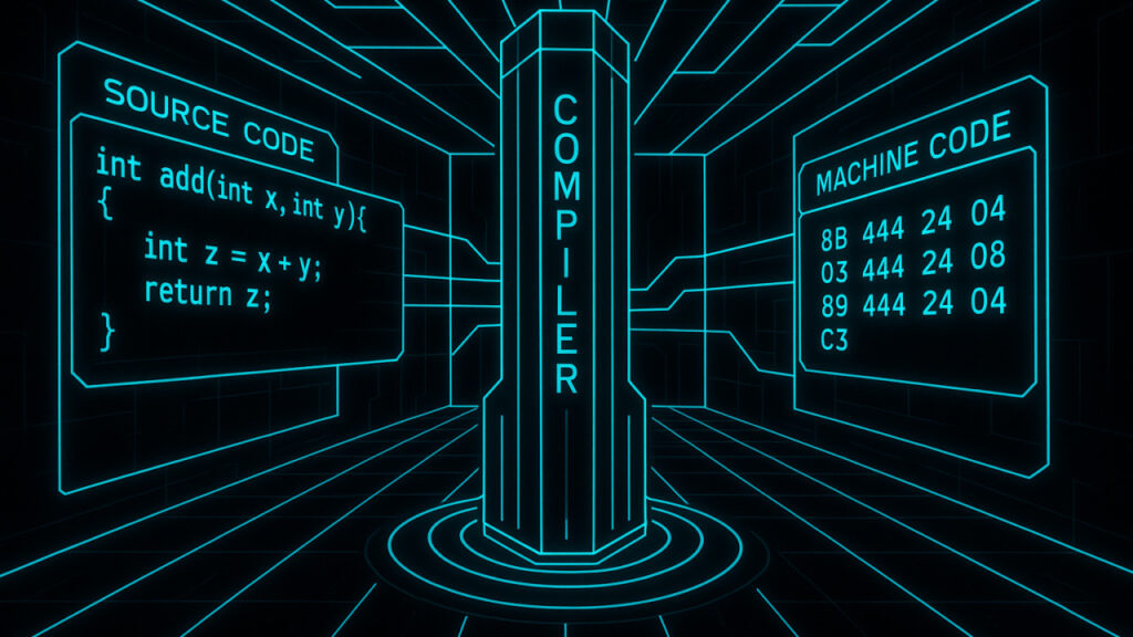
Let’s start with the basics. The way that computers work is that the CPU takes machine code (CPU instructions and operands that the CPU can use) and runs it. Machine code goes by many names: binaries, executables (EXE files on Windows), etc. When you go to run a program, the executable is loaded from file storage into memory, and the memory controller feeds the machine code to the CPU. If you were to open up machine code in a text editor, it’d look like gibberish. Machine code comes in different flavors as well, as it’s specific to the CPU it’s meant to run on. x86-64 machine code looks different than ARM machine code, for example.

The task at hand is then to convert the control program’s human-readable form (the source code, written in a PL) so the system can run it. How do we do that?

Well, there are a few main ways to implement this:

• Run on an interpreter: A specialized program called an interpreter reads the source code of your control program line by line (or rung by rung) and does all the actions directly. As you might imagine, this is very slow and inefficient because the interpreter has to read the source code (with long tag names the computer doesn’t care about) and figure out what to do every single time. Examples of this are running VBA macros in Microsoft Excel, and (showing my age) running a BASIC program back in the MS-DOS days.
• Run on a bytecode virtual machine (VM): This is like using an interpreter, but faster and vastly more efficient. In this mode, a specialized program called a bytecode compiler reads your source code and converts it to a special bytecode or intermediate representation, which is basically a shorthand version of your source code. This bytecode is then fed into a bytecode VM, which operates similar to a CPU (but in software, hence the name virtual machine). The VM reads the bytecode and does all the required actions. The source code only needs to be compiled to bytecode once. Examples of this are the default implementation of Python (CPython), and most PLCs.
• Compile and run directly: A specialized program called a compiler reads your source code and converts it directly to machine code which can be run directly on the CPU. The source code only needs to be compiled to machine code once. This is called Ahead-of-Time (AOT) compilation. This is the fastest option with the least amount of overhead. PLs that usually do this include: C/C++, Rust, etc.

To give a better idea on speed, bytecode interpretation might be 5-20x slower than a program that is compiled AOT, while regular/pure interpretation might be 10-100x slower. Results may and will vary.

It’s not always so black and white, as there are other ways and combinations of the different options. Some interpreters and bytecode VMs use Just-In-Time (JIT) compilation to convert some source code into native machine code when the program is run so that it can run faster. Examples of this are the Java and .NET runtimes.

The thing is this: programming languages are just that, languages. Think of them as specifications and instructions for something that needs to be done.

Let’s look at Python again. The reference implementation, CPython, is a bytecode compiler/VM. When you run a Python script, the .py file is compiled into bytecode and stored as a .pyc file with the same name. Then, CPython loads the .pyc file and runs it. So, when people are saying that Python can’t deliver scan times less than 1 millisecond, they’re probably referring to the performance they’ve seen from CPython. But, this is not the only way you can run a Python program. There are other implementations that can run Python programs dramatically faster:

• PyPy, a JIT compiler
• Codon can be used as both a JIT and AOT compiler, as well as a bytecode compiler
• Cython transcompiles (converts one PL to another) Python into C/C++ so that it can be compiled to machine code

With these alternate implementations, a Python program with a control loop could easily achieve scan times less than 1 ms (on a modern ARM or x86 CPU). This is in comparison to typical PLC scan times which can be ~3-5 ms on average.

As for reliability, again, implementation specific. If you use a PL implementation that’s incomplete or buggy, then you’ll get unreliable programs in return. Businesses all over the world are running programs written in all kinds of different PLs on servers that need to maintain virtually 100% uptime. For that reason, it’s smart to use long-term support (LTS) versions of software that emphasize stability and lack of bugs / security vulnerabilities over new features.

#5 – Deterministic / real-time execution:

Keeping timing predictable is a function of what’s done in the program regardless of the PL, and as covered already, how the operating system is set up. Since we’ve already covered operating system setup, let’s talk about what things can get you into trouble. In a nutshell, it’s memory management and I/O calls that can cause unpredictable delays and jitter.

Regarding memory management, one of the things that can cause issues that’s mentioned often in these discussions (which is absolutely true) is garbage collection. Garbage collection is when the program de-allocates/frees dynamically allocated memory that falls out of scope, i.e., is not needed anymore. Both garbage collection and the dynamic memory allocation itself can cause delays.

To dig a little deeper into what’s going on with dynamic memory allocation, we need a little background on program memory. A program’s memory comes from two places called the heap and the stack. You could write entire articles on both of these so we’ll keep it simple, but the stack is basically a finite amount of memory statically allocated for the program that is easily accessible, while the heap is basically free system memory that can be allocated dynamically during program execution. Data structures that have set sizes known ahead of runtime are placed in the stack, while anything determined on-the-fly comes from the heap.

With that background, back to memory allocation/de-allocation. When a program requests some of that free system memory from the heap, the system has to find where it can be put and if it has to break it up into chunks (memory fragmentation). Basically, for that reason, either requesting or freeing dynamic memory is a no-go here. So what do you do instead? Just declare data structures with set sizes, big enough to cover all use cases. You can get fancier than that, but that would be the easiest way.

Regarding I/O, if the program has to sit and wait for another device to respond (could be a local storage device like a hard drive, another device on the network, a serial device, etc.) then by definition timing is going to be erratic. Sitting and waiting for something to respond is called blocking I/O because it blocks the program’s execution until it receives what it’s waiting for. The solution, which is what PLCs do of course, is to use non-blocking I/O. The program chooses when to trigger the I/O in the case of manually sending a message, but the I/O system sitting in the background is the one stuck doing the waiting instead of the main program, and it lets the main program know once the data is ready. In the case of accessing system memory on a PLC, that background I/O system is silently waiting for connections to be made and synchronizing with the program’s memory.

Obviously, it can be more complicated than all that, but to wrap-up: if you stay away from the obvious things that will cause unpredictability (and the OS is set up correctly), you can expect deterministic execution.

Conclusion

A lot of information was covered in this article, perhaps too much. Hopefully though this has been informative and if there’s one thing to leave with, it’s to realize that programming languages themselves are just like specifications–how you implement those specifications is everything.